Calculating Stock Correlations

A toy project that explores visualising stock return correlations

Author

Jason Lee

import pandas as pd
import yfinance as yf
import seaborn as sns
import matplotlib.pyplot as plt

Downloading Stock Data from yfinance

universe = pd.read_csv("../data/universe.csv")

# Date range
start = '2021-01-01'
end = '2024-09-22'

# Tickers of assets
assets = universe['Ticker'].to_list()
assets.sort()

# Downloading data
data = yf.download(assets, start = start, end = end)
data = data.loc[:, ('Close')]
data.columns = assets

data

[                       0%                       ][*****                 10%                       ]  2 of 20 completed[*******               15%                       ]  3 of 20 completed[*******               15%                       ]  3 of 20 completed[************          25%                       ]  5 of 20 completed[************          25%                       ]  5 of 20 completed[*****************     35%                       ]  7 of 20 completed[*******************   40%                       ]  8 of 20 completed[**********************45%                       ]  9 of 20 completed[**********************50%                       ]  10 of 20 completed[**********************55%*                      ]  11 of 20 completed[**********************60%****                   ]  12 of 20 completed[**********************60%****                   ]  12 of 20 completed[**********************70%*********              ]  14 of 20 completed[**********************75%***********            ]  15 of 20 completed[**********************80%*************          ]  16 of 20 completed[**********************85%****************       ]  17 of 20 completed[**********************90%******************     ]  18 of 20 completed[**********************95%*********************  ]  19 of 20 completed[*********************100%***********************]  20 of 20 completed

	ACWX	BND	DBC	EWJ	FLIN	FXI	GLD	INDA	IWV	QQQ	REET	TIP	VCN.TO	VEU	VGK	VGT	VNQ	VTI	VXF	XIU.TO
Date
2021-01-04	47.711861	78.622475	13.149570	61.875252	25.043995	42.370186	182.330002	37.514973	209.478271	301.685425	20.478315	109.025612	31.250051	51.620850	53.464718	337.758484	70.930550	180.991165	154.595184	23.268791
2021-01-05	48.409817	78.488556	13.518332	62.449890	25.429298	43.523239	182.869995	38.194351	211.254089	304.172607	20.566353	108.991486	31.570019	52.412983	53.946621	340.535034	71.034149	182.453293	156.872391	23.490656
2021-01-06	48.615627	78.140388	13.536322	63.191364	25.371410	43.019924	179.899994	38.073364	212.877960	299.959045	20.733633	108.667290	31.845545	52.694630	54.586227	334.884857	71.154999	184.094650	160.254929	23.721390
2021-01-07	48.875122	77.979713	13.599280	63.061596	25.377102	43.321915	179.479996	37.896542	216.363068	307.215698	20.583963	108.599022	32.218838	52.879459	54.752712	344.418365	71.016884	187.047134	163.599319	24.005369
2021-01-08	49.537296	77.908310	13.707211	64.220139	25.889584	44.218739	173.339996	38.789978	217.512161	311.165833	20.724831	108.172478	32.227726	53.627590	55.006802	346.932770	71.707451	187.952713	163.856567	24.040869
...	...	...	...	...	...	...	...	...	...	...	...	...	...	...	...	...	...	...	...	...
2024-09-16	54.599186	74.711632	20.714136	69.455086	41.408691	25.626524	238.660004	57.712471	318.677185	471.815094	26.472399	110.249245	47.879375	60.079185	69.305176	564.339111	97.203011	276.027222	177.350891	35.702126
2024-09-17	54.411861	74.612862	20.856533	68.637848	41.279507	25.951660	237.339996	57.543690	319.015076	472.064362	26.277531	110.209442	47.795544	59.844006	69.048706	564.049866	96.525330	276.305450	178.265686	35.612873
2024-09-18	54.273834	74.385681	20.723629	68.322769	41.021137	25.803871	235.509995	57.245846	318.041168	470.020538	26.199587	109.801559	47.657463	59.667614	68.881020	561.447083	96.407478	275.609863	178.325333	35.483948
2024-09-19	55.348469	74.385681	21.093864	70.134476	41.339130	26.730011	239.169998	57.692612	323.606384	481.904633	26.287275	110.129860	48.190056	60.814129	70.074570	578.051208	96.427124	280.280334	181.885086	35.890553
2024-09-20	54.944248	74.375809	21.093864	70.173851	41.985054	26.749716	242.210007	58.318089	322.741791	480.987396	26.141127	109.980637	48.197994	60.427479	69.027435	576.026733	96.044083	279.694061	180.681946	35.900475

954 rows × 20 columns

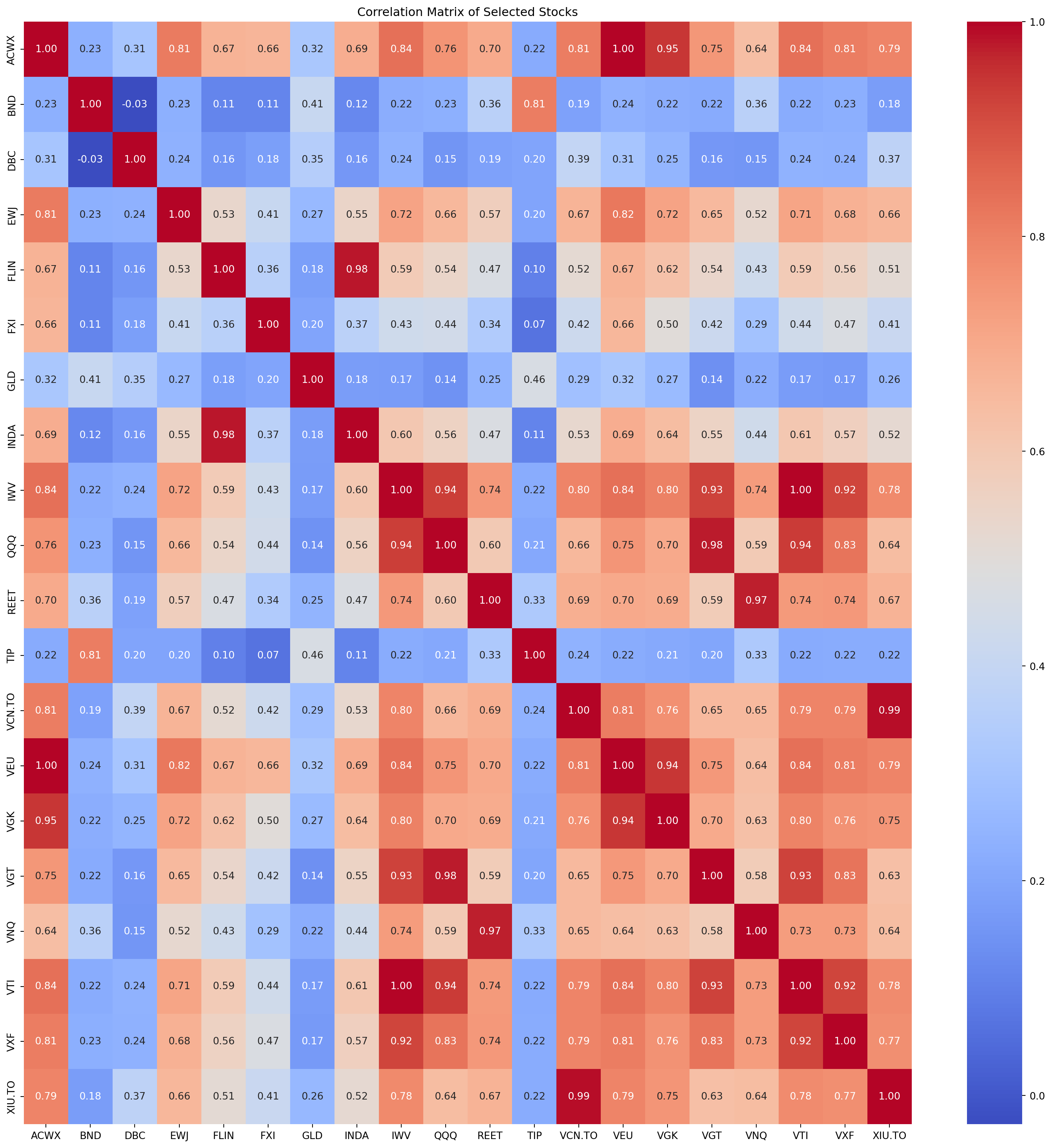
Calculating stock returns and correlation

#Calculating Returns
returns = data.pct_change().dropna()

correlation_matrix = returns.corr()

# Plot the heatmap
plt.figure(figsize=(20, 20))
sns.heatmap(correlation_matrix, annot=True, cmap='coolwarm', fmt=".2f")
plt.title('Correlation Matrix of Selected Stocks')
plt.show()

/var/folders/49/wztx6mrd3qd9qcgjnk_y96040000gn/T/ipykernel_97769/4222160605.py:2: FutureWarning:

The default fill_method='pad' in DataFrame.pct_change is deprecated and will be removed in a future version. Either fill in any non-leading NA values prior to calling pct_change or specify 'fill_method=None' to not fill NA values.